When I was a graduate student, I studied the growth of large sharks by staining and counting growth bands in vertebral centra (much as one would count tree rings to determine age). I was impressed that some sharks could live over 30 years and thought this must be telling me something about mortality rate. But, what?
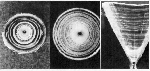
From left to right: whole vertebral centra of smooth dogfish and lemon shark, and polished section of a lemon shark centrum, stained using cobalt nitrate and ammonium sulfide according to a procedure developed by Hoenig and Brown (1988).
One day I plotted values of natural mortality rate versus oldest age known for whatever fish, mollusk and cetacean species I could find in the literature. The plot looked linear (on a log - log scale) and suggested that one can get a rough idea of the mortality rate if one knows the maximum age.
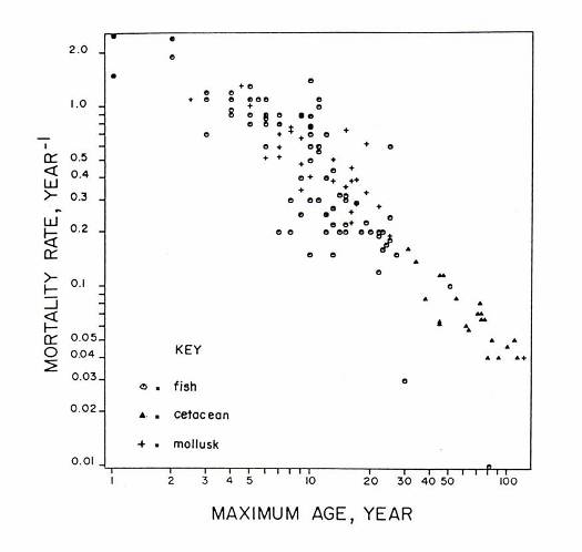
Plot of natural mortality rate (log scale) versus maximum age (log scale), from Hoenig (1983).
This simple paper has been a "best seller". According to Google Scholar (http://scholar.google.com), it has been cited 228 times (as of 5/1/2007). Many stock assessment models use a value of natural mortality computed from my regression formula. Interestingly, the first time I submitted it for publication it was rejected. (The reviewer sniffed that it was just another example of life history correlates.) But, I immediately sent it to another journal and it was accepted. It is somewhat humbling that my best cited work was developed as a side project while I was a graduate student.
Another "best seller" is my 2001 paper with Dennis Heisey on the inappropriate use of power calculations as a data analytic tool. We found over 20 peer reviewed articles in the applied scientific literature that indicated that whenever a statistical test fails to reject the null hypothesis one should, indeed one must, do calculations of statistical power. Some journals even required such power calculations. The proponents of this approach argued that one must distinguish between the case where the statistical power was low - so it is possible the null hypothesis was false but one didn't have the power to detect this - and the case where the statistical power was high - so if the null hypothesis were false one probably would have detected this. Thus, the computed statistical power was viewed as a way to determine whether the null hypothesis should be accepted (or viewed as credible and likely to be true) although the proponents of this technique were never clear exactly how one uses the computed power. This seemingly reasonable approach is logically flawed. It turns out that the computed power is a one-to-one function of the p value obtained for the test. Thus, the computed power brings forth no new information; it is just a re-expression of the p value. To illustrate, suppose one does a one-sided Z test to compare a mean to a theoretical value for the mean. Suppose the result turns out to be marginally (non-)significant, e.g., p = .05001. Then, without even knowing the sample size, the estimated effect size, or the standard error, we can determine that the "observed power" was 0.5. Thus, we cannot judge whether this particular null hypothesis is credible by looking at the observed power for this particular experimental outcome: given that the result is marginally significant the observed power is fixed.
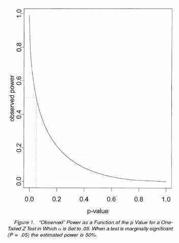
The main points are that statistical power computations are useful for planning a study but provide no new information to aid in the interpretation of non-significant test results. What should one do if a statistical test outcome is non-significant? We suggest the investigator compute confidence intervals about the parameter estimates. These intervals provide the range of possible parameter values that cannot be refuted by the data.
The controversy over power calculations arose, I believe, from a concern about who should bear the burden of proof in an investigation. Historically, scientists adopted the idea that scientific conclusions should not be admitted into the body of scientific knowledge unless the investigator could "prove" in some sense the validity of the result. However, there are many cases where this is not the intention of the scientists or the society. For example, consider the construction of a new power plant along a river. This plant could be very useful to society but there is also the potential that it will cause environmental harm. It may be necessary to build cooling towers to protect the riverine ecosystem. The power company, the investors, and the Chamber of Commerce may wish to build the plant without towers unless it can be shown to be harmful. The environmentalists might wish to block the operation of the plant unless it can be shown to be environmentally friendly. Both viewpoints are rational. They reflect the differences of opinion in society as to who should assume the burden of proof.
Statistical tests can be designed to place the burden of proof where it is desired. Suppose we want to determine whether the power plant is raising the water temperature more than 5 degrees during the summer because it is believed summer temperature elevations greater than 5 degrees are harmful. The power plant advocates would want to test the hypothesis
Ho: temperature rise < 5 degrees
versus the alternative
Ha: temperature rise > 5 degrees.
Thus, if we reject the null hypothesis the power company has to install cooling towers; otherwise the plant can be operated without towers.
The environmentalists want to test the following hypothesis:
Ho: temperature rise > 5 degrees
Ha: temperature rise < 5 degrees.
Thus, the plant cannot be operated unless the null hypothesis is rejected, i.e., the burden is to prove the plant is safe.
How does this matter? Consider the viewpoint of the advocates of operating the power plant without cooling towers. If the first set of hypotheses is adopted for testing, the advocates of operating without towers will want to argue for as small a sample size as possible to keep the power low so the null hypothesis is not rejected. On the other hand, if the second set of hypotheses is adopted for testing, the advocates of operating without cooling towers will want as large a sample size as possible so that they have a good chance of rejecting the null hypothesis that the plant is harmful in favor of the alternative hypothesis that the plant is benign.
Our paper appeared in 2001 and already it's been cited 122 times in the peer reviewed literature (according to ISI's Web of Science, which keeps track of citation rates). Counting gray literature and web citations, it's been cited over 150 times (according to Google Scholar).
I've been interested in the elasmobranchs (sharks, skates and rays) since graduate school days when I studied growth rates and longevity of sharks (see What does longevity imply about mortality?). After graduate school, I was fortunate to be able to spend two years at the Rosenstiel School of Marine and Atmospheric Science where I worked with Samuel (Sonny) Gruber on lemon sharks. We used a Leslie matrix model to predict that lemon sharks have a survival rate during their first year of life of around 50%. We also showed how the Leslie matrix modeling approach could be used to estimate an upper bound to the amount of fishing mortality that is sustainable (see Hoenig and Gruber 1990 ).

My colleague Samuel (Sonny) Gruber with a juvenile lemon shark in Bimini, Bahamas.
We later verified the prediction of a 50% survival rate for young of the year lemon sharks by conducting a novel mark depletion study on juvenile lemon sharks in Bimini Lagoon in the Bahamas. Furthermore, we found that the first year survival rate was very much linked to the abundance of pups: in years with fewer pups born the pups had a higher survival rate than in years in which pups were abundant (see Estimation of survival rates of juvenile lemon sharks in Bimini, Bahamas with Sonny Gruber and Jean DeMarignac).
The approach to using Leslie matrices to set limits to sustainable fishing mortality has turned out to be an important tool for management of elasmobranch stocks. However, many people have misinterpreted the model. This prompted my graduate student Todd Gedamke and me to write a paper about the pitfalls of using demographic analyses and to show how the field can be advanced (see Gedamke et al. 2007).
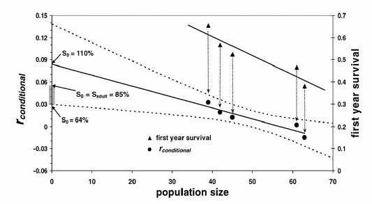
This graph shows (top right) the estimates of first year survival of lemons sharks we obtained in Bimini and the corresponding population size (number of pups present immediately after the pupping season). Survival decreases from about 60% when there are 40 pups present to about 40% when there are 60 pups present. Each first year survival estimate can be plugged into a Leslie matrix model to calculate the corresponding rate of population growth (assuming all other parameters are known and fixed). The rate of population growth can be extrapolated back to zero population size to obtain an estimate of maximum (intrinsic) rate of population growth. In this case, the estimate is 0.09 yr-1. However, this rate of growth would imply a first year survival of 110% which is not possible. We assume that first year survival rate cannot rise above the survival rate of adults in an unfished situation (i.e., around 85%). If we fix the first year survival rate at 85% we obtain a rate of population growth of around 5.5%. This is probably an upper bound. On the other hand, if we use the lower limit to the 95% confidence interval on the rate of growth at zero population size, we obtain an estimate of maximum growth rate of 3% yr-1. Thus, the available information suggests that the maximum population growth rate for lemon sharks is in the range of 0.03 to 0.06 per year (shaded rectangle along the y-axis). It may seem unimpressive that the extrapolation back to zero population size produced an infeasible estimate of population growth. But, it should be remembered that this is the first time such calculations are being made and the procedure has a built in mechanism for testing the reasonableness of the predictions. To our knowledge, no one else is devising methods to test elasmobranch model outputs.
The focus of Todd Gedamke's dissertation, however, was on barndoor skates off the Northeast United States coast. The National Marine Fisheries Service (NMFS) trawl survey indicated that barndoor skates were common in the early 1960s, they largely disappeared in the 1980s and early 1990s, and then began rebounding in the mid-1990s. The regression line at the far right suggests the skate population was growing at an instantaneous rate of 0.36 per year in the 1990s. This rate of growth is presumably determined in part by how much fishing mortality there is and how large the population is (in theory, as a population is reduced in size its potential growth rate increases). Todd's work involved correcting the observed population growth rate to remove the effects of fishing and extrapolating the resulting growth rate back to zero population size.
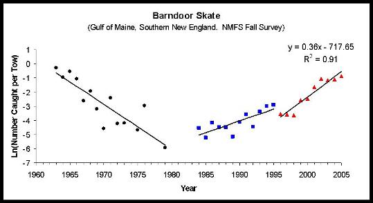
The techniques we developed are now being applied to several other species of skates off the northeast coast in order to assess stock status and develop fishery management plans.
The National Marine Fisheries Service (NMFS) conducts a research survey each year to estimate the abundance of sea scallops. It then sets a catch quota as a specified fraction of the estimated abundance.
The estimation of scallop abundance can be thought of as consisting of two steps. First, a swept area calculation of dredgeable biomass is obtained. This consists of estimating the average catch in the survey dredge per square kilometer of bottom swept by the dredge. This raw density estimate is then multiplied by the total area being surveyed to obtain a minimal estimate of biomass. The minimal estimate is then corrected for the fact that the survey dredge is not 100% efficient.
It is important to estimate the survey dredge efficiency, which is the fraction of the scallops encountering the gear that is retained by the gear (some scallops may escape under the dredge or pass through the dredge). The actual abundance estimate is obtained by dividing the dredgeable biomass estimate by the gear efficiency. NMFS scientists argued the dredgeable biomass should be divided by a number around 0.40. Industry scientists argued the number should be around 16%. Obviously, the closer the number used for dredge efficiency is to zero, the larger the estimate of actual abundance becomes.
My student Todd Gedamke spent 78 days at sea on commercial scallop boats collecting data on area swept and catch on a tow by tow basis. He also obtained vessel monitoring system data, observer data, and survey data from the National Marine Fisheries Service Woods Hole Laboratory.
 |
 |
Todd Gedamke's adventures at sea
while conducting research for his Master's thesis. |
|
Todd was able to estimate the gear efficiency two ways. One way was to use an index-removal estimator. It works this way. Suppose the catch rate is 20 bushels per standard tow before the fishery opens, and suppose 5 million pounds of scallops are harvested during a fairly short fishing season. If a survey conducted after the fishing season and the catch rate is 10 bushels per tow, then we can imagine that a 50% reduction in catch rate (from 20 to 10) implies that 50% of the population has been harvested. Hence, 5 million pounds was half the population so the initial population was 10 million pounds. This assumes that catch rate is proportional to abundance, that there is no recruitment, emigration or immigration during the fishing season, and there is no natural mortality during the fishing season. These assumptions may be quite reasonable if the fishery is of short duration. More formally, the population size can be estimated by
Population Size = R c1 / (c1 - c2)
where R is the removal (e.g., 5 million pounds), c1 is in pre-season catch rate (e.g., 20 bushels/tow) and c2 is the post-season catch rate.
Todd also used a DeLury depletion estimator to estimate population size. This consists of examining how the catch rate declines over the season as the cumulative fishing effort increases. This is an old technique and it can provide misleading results when applied to commercial catch and effort data unless care is taken to meet the assumptions. In particular, what often happens is the fishers start fishing close to port on high concentrations of scallops. But, as they start to deplete the scallops, they move on to other areas to keep their catch rates up. Thus, instead of seeing a steady decline in catch rate, one is likely to see very little decline until possibly the end of the season when there are no unfished areas left and areas begin to be fished for a second and third time. Todd was able to overcome this problem by defining a set of cells covering the scallop fishing grounds and sifting through massive amounts of records to identify a small set of grid cells in which the assumptions of the DeLury method appeared to be met. Thus, he required that each quarter of a grid cell was fished in both the first and second half of the season, that the fishing effort in the cell was substantial, and that there were observer records of catch rates in both the first and second half of the season.
The index-removal and DeLury depletion methods provide estimates of population size. They can also provide estimates of the catchability coefficient, q, which is the fraction of the population caught by one unit of fishing effort. That is,
catch per tow = q N
where N is the abundance at the start of the fishing season.
The gear efficiency, e, is related to the catchability coefficient, q, by the equation
q = a e / A
where a is the area swept by one unit of fishing effort and A is the total area inhabited by the stock.
Using this approach with the index-removal and DeLury estimates of abundance, Todd found the efficiency of the scallop dredge to be around 50%, close to the value adopted by the National Marine Fisheries Service.
My student John Walter found Todd's work interesting and pursued the ideas further. John was interested in spatial modeling of the scallop population and the scallop fishery. In particular, he wondered what inferences could be made when data are not collected according to a randomized sampling design but, rather, are collected in a biased manner. The idea is that massive amounts of data on commercial fishing activities are available; the trick is to find a valid way to interpret these data. John used the geostatistical technique known as kriging to construct maps of scallop effort, abundance, and gear efficiency.
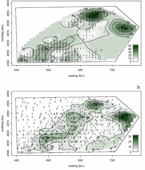
Kriged maps of scallop abundance on Georges Bank Closed Area 2. Top map is based on observer data collected during the fishing season. Bottom map is based on NMFS pres-season survey data.
The relative abundance of many crustacean stocks is assessed by examining the catch rate in pots (traps) deployed in a research survey. The catch is often divided into several groups (e.g., legal size vs. sublegal size, male vs. female) so that trends in abundance over time can be tracked separately for each component of the population.
My student, Stewart Frusher, worked on assessment of southern rock lobster (Jasus edwardsii) stocks in Tasmania, Australia. He noticed that there was a negative correlation between the catch of legal size and sublegal size animals. Now, this would be expected if the pots fill to capacity because a large catch of large animals would leave little room for small animals, and vice versa. But, lack of space in the pots does not explain what Stewart saw. Stewart wondered if there was some kind of behavioral interaction whereby large lobsters inhibit smaller ones from entering pots.
Stewart conducted an experiment in a small reserve off the Tasmanian Aquaculture and Fisheries Institute in Taroona (near Hobart). He set pots every day and when he hauled the pots he removed all of the catch and brought the animals back to holding facilities at the lab. As might be expected, as he expended more and more cumulative effort, the catch per pot of large animals dropped off, presumably because he was depleting the large lobsters. But, what he saw with the sublegal size animals was quite interesting. In the beginning, the catch per pot of small animals was quite low. As the experiment progressed, the catch rate of small lobsters rose to a peak. Towards the end of the experiment, the catch rate of small lobsters dropped off.
 |
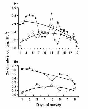 |
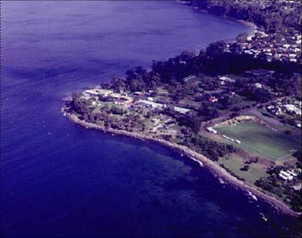
| The Marine Reserve off Crayfish Point, where the Tasmanian Aquaculture and Fisheries Institute is located. | Results from two surveys conducted in 1999 in the lobster reserve adjacent to the Tasmanian Aquaculture and Fisheries Institute. In each survey, 50 pots were set and hauled after 24 hours, and all lobsters were taken to holding facilities on shore. Solid symbols denote the catches of large lobsters and open circles denote catches of small lobsters. Note the dome-shaped curves for small lobsters. |
These results are suggestive of the idea that initially the abundance of large lobsters was high and this inhibited small lobsters from entering the traps. As the large lobsters were depleted, the smaller ones entered the traps and were caught. Eventually, the catch rate of smaller lobsters dropped off as the population of small lobsters was depleted by trapping. Stewart devised several other ways to investigate this hypothesis which are described in Frusher and Hoenig (2001).
These results have important implications for stock assessment and fishery management (Frusher et al. 2003). Suppose that over a period of years the abundance of large lobsters is gradually reduced, as determined by a research pot survey, but the abundance of small lobsters in the survey appears stable over the years. If the theory that large lobsters inhibit smaller ones from entering traps is true, and if the abundance of large lobsters has been reduced, then constant recruitment over time would imply that the catch rate of smaller lobsters should rise over time in the survey. If, instead, the catch rate of small lobsters remains constant, then this would imply a reduction in recruitment over time (which is being masked by the behavior interaction between large and small lobsters).
My student Tom Ihde was intrigued by these results and decided to pursue the investigation further. He conducted experiments in which he fished pots, some of which contained just bait, and some of which contained a large lobster. He wanted to see if the pots seeded with a large lobster caught less than the traps without the seed. His results suggest that behavioral interactions may be complex and may vary with the season (see Ihde, Frusher and Hoenig. 2006. Do large rock lobsters inhibit smaller ones from entering traps? - a field experiment. Mar. Freshwater Res. 57:665-674.)
Bycatch - the unintentional catching of unwanted animals - is a major problem in many fisheries. Very little of the discarded bycatch is thought to survive. Thus, bycatch represents a waste of resource. To the extent that bycatch losses to the stock are not quantified carefully, they also represent a major uncertainty in the assessment of stock status. In some fisheries, the management regulations specify that the fishery will be closed when either the catch quota or the cap on bycatch is reached. An example is the fishery for sea scallops on Georges Bank (off Massachusetts) which is shut down when either the quota for sea scallops or the bycatch cap on yellowtail is reached.
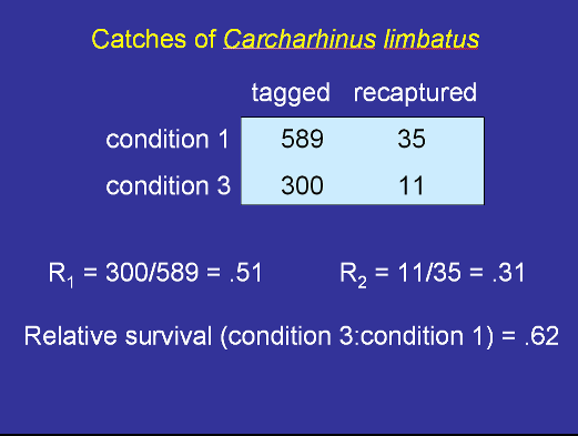
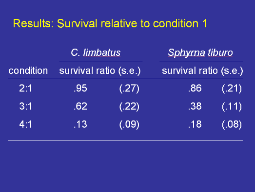
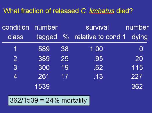
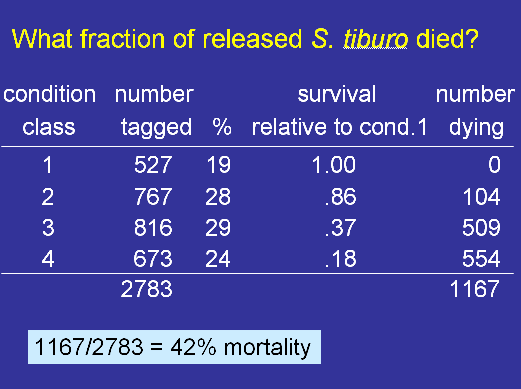
My colleagues at Mote Marine Laboratory and I recently published a paper that shows how discard mortality can be quantified using tag return data (see Hueter et al. 2006). Sharks were captured in a gillnet fishery (the fishery has since been closed), and the animals were tagged, and released. The novel aspect of the study was that each animal was assigned a condition category at the time of release with Condition 1 representing animals that showed no stress or effects of capture (they swam off vigorously when released) and Condition 4 representing animals in poor condition.
If the condition has no bearing on the survival of the discarded animal, then we would expect to obtain the same proportion of tags returned from each condition category. But, suppose that we get tags back from 5% of the animals in condition 1 and only 2% from animals in condition 2. Then we would infer that animals in condition 2 have 2/5 = 40% of the survival rate of animals in condition 1. Furthermore, if we assume that all animals in condition 1 survive, then we can infer the survival rate of discarded animals in condition 2 is 40%. That is, the 40% figure can be interpreted as an absolute rate and not just a relative rate.
The study found the following for the blacktip shark (Carcharhinus limbatus) and the bonnethead (Sphyrna tiburo).
All fishing gear is size-selective, meaning that some sizes of fish are more catchable than others. This has important implications for fisheries management. First, we use catches in surveys to get a picture of the size composition of the population. In order for this picture to be accurate, it is necessary to know how size-selectivity affects the survey catches. Second, the amount of yield obtained from a fishery depends on how much fishing activity occurs and the selectivity of the fishing gear. Adjustments to the gear, such as changes in mesh size, can affect the potential yield from the fishery.
My colleague Ransom Myers and I developed a simple method for estimating size selectivity using tagging data. An important feature of the method is that it allows data from various studies to be combined. Here, I give the simplest explanation of the method. The interested reader should consult the paper (Myers and Hoenig 1997).
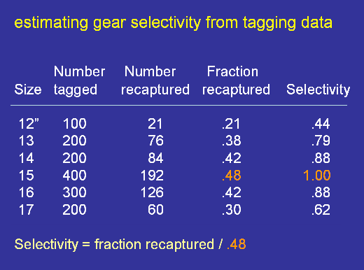
Suppose we tag and release fish of various sizes and then count the number of tag returns we get over the next few months. (We keep the time interval short so that we don't have to deal with the complication of fish growing to larger sizes and thus having changing selectivity.) If the gear is non-size-selective, then we should expect to get back the same percentage of tags from each size group (except for random sampling error). To the extent that we get a lower percentage of tags back from some size groups we have size selectivity. In the table below, we can see that the 15 inch size group has the highest rate of return (48%). By convention, we assign this size group a selectivity of 1.0 and then construct the selectivity curve by dividing the proportion of tags recovered from each length interval by 0.48.
We applied this technique (in a slightly more complicated form) to tag return data for cod from NAFO (Northwest Atlantic Fisheries Organization) area 2J3KL.
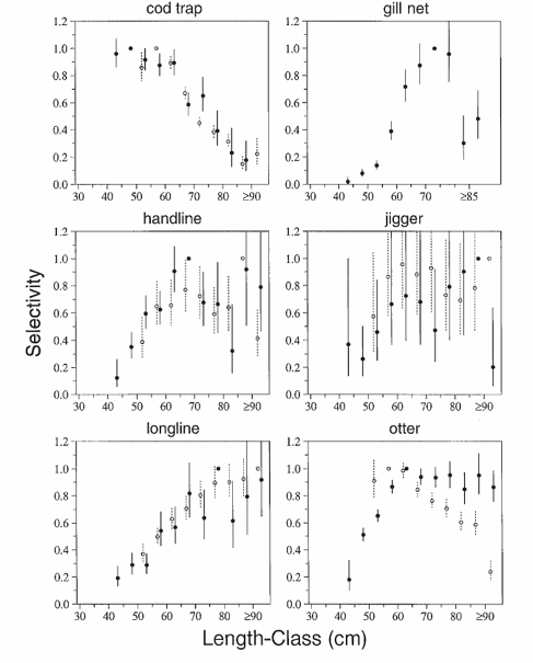
Estimates and standard errors of gear selectivity for Atlantic cod off Newfoundland, Canada, from 1954 to 1964 (open circles) and from 1979 to 1990 (solid circles) versus the length at tagging. The selectivity for each gear type is standardized so that the length-class with the maximum selectivity has selectivity equal to one. There will be no standard error associated with this selectivity. Data for fish longer than 90 cm have been pooled. For cod traps from 1979 to 1990 we combined all data over 85 cm because there were very few returns for cod longer than 85 cm. Gill-net selectivity is estimated from fish tagged after 1978 with spaghetti tags. From Myers and Hoenig (1997).
From the above graph, we can see that cod traps select for small fish while handlines and longlines select for large fish. The gillnets have a dome-shaped selectivity curve, as is typical for gillnets. The data for jiggers were not very extensive so we really don't have a very good idea of the selectivity of fishing with jiggers.
The selectivity curves for otter trawls are extremely interesting. In the early years, the curve was what dome shaped while in more recent years it was "flat topped". This makes sense. In the early years, wooden boats with smaller engines were used and the trawl was deployed over the side of the vessel; in contrast, in more recent years, steel hulled vessels with larger engines were used, and the trawl was deployed over the stern. Thus, it is likely that in the earlier years, large cod could avoid the oncoming trawl while in later years they couldn't.
Anadromous fishes spend most of their lives in the ocean and return to their natal river only to spawn. While at sea, the stocks often mix so that an ocean fishery may catch fish originating from several rivers. I'm interested in the stocks of American shad that spawn in Virginia's rivers. It is known that there is a high degree of fidelity to the natal rivers so each river has a distinct stock. Unfortunately, Virginia's and Maryland's shad stocks have declined substantially so there is currently a moratorium on fishing for American shad in Chesapeake Bay and its tributaries.
The American shad was historically one of the most important anadromous fishes in the United States. Since the late 1800s however there has been a steady decline in the abundance of American shad along the Atlantic coast. This decline in landings has been attributed to several factors including overfishing, construction of dams, and pollution.
An important question is what is the impact on individual river stocks of a fishery harvesting a mixture of stocks in the ocean. I developed a rather clever method with my colleagues at VIMS, John Olney and Rob Latour, to estimate the fraction of a mixed-stock catch coming from the York and the James rivers.
The method takes advantage of the efforts under way to restore the shad stocks in the York and James rivers. Hatchery-reared larvae are given a river-specific mark by immersing them in an oxytetracycline bath on specific dates to create a pattern of fluorescent bands in the otoliths. These larvae are then released into the rivers where they join their wild counterparts and migrate out to sea as juveniles. We obtained otoliths from the offshore mixed-stock catch and also from adults subsequently returning to the York and James rivers to spawn.
Suppose 4% of the offshore mixed-stock catch has a James River mark. If 100% of the offshore catch is from the James River, then when we sample adults in the James River 4% of them should have marks. What if only half of the offshore catch is from the James River? Then there is a 50% dilution of James River marks in the offshore catch. Consequently, sampling adults in the James River should show that 8% of the spawners have marks.
This can be formalized as follows:
f = p/p
where f is the fraction of the offshore catch that is from the James River, is the fraction of the offshore catch with James River marks, and p is the fraction of the spawners swimming up the James River that have marks.
The data we collected look like this:
| # caught | # marked | proportion marked | |
| Offshore catch (2000) | 192 | 1 | 0.52 % |
| In-river monitoring (2000) | 387 | 156 | 40.31 % |
| Offshore catch (2001) | 594 | 4 | 0.67 % |
| In-river monitoring (2001) | 256 | 103 | 40.23 % |
Thus, we estimate that 1.29 % of the offshore catch was from the James River in 2000 and 1.67 % was from the James in 2001.
A very interesting aspect of this estimator is that one does not need to know how many marked larvae were released into each river. Very few models for tagging data can handle the situation where the number marked is unknown.